Friday, October 24, 2014

Pixel-Based Supervised Classification

- Introduction and Background -

To perform supervised classification, an analyst will collect samples areas of known land cover, commonly referred to as training samples, from the image which will be used to train a classifier. The classifier will then classify the entire image based on the information gathered from the collected training samples. Preferably, training samples would be collected based on prior knowledge of the area using the most accurate means available (GPS, topographic survey, etc.) However, for some applications this is impractical and high resolution imagery can be used to designate areas for training samples.

Important factors to consider when collecting training samples include: the number of training samples, the number of pixels, shape, location, and uniformity. In general, a minimum number of 50 training samples per informational class is required to produce an accurate classified LULC image. The specific number of training samples for individual informational classes may vary depending on the nature of the image (spectral diversity) and project (special emphasis or resource availability). Another factor that may fluctuate is the number of pixels. Generally, 10n pixels, where n is equal to the number of bands in the image, is required to provide enough spectral information for the training sample's informational class to be properly identified. The shape of training samples will normally be a derivation of a polygon. Training samples should be distributed throughout the entire image to account for spectral variability in the informational classes and be located within a uniform and homogeneous land cover. An important concept to keep in mind is the geographic signature extension problem where differences in spectral characteristics of the same informational class result form differences from a variety of factors like, soil moisture and type, water turbidity, and crop species. To reduce the errors that result from the geographic signature extension problem, training samples should cover all possible variations of the desired informational classes (e.g. for vegetation, collect forest and riparian vegetation).

Training samples need to be evaluated before they are used to train a classifier. The histograms of a training sample should not be primarily multimodal. Training samples with more Gaussian histograms will produce a more accurate classified LULC image. If a training sample exhibits mostly multimodal histograms it should be deleted and collected again. Spectral separability will indicate the best bands to use for an analysis based on the separation of the bands of the spectral signatures of the training samples. The larger the separation between spectral signatures for a particular band, the better that band will be for classifying different land covers. Spectral separablilty can be calculated using software like ERDAS IMAGINE and produces a list of the best bands and an average score. The maximum value of the average score is 2000 indicating excellent separation between classes. Values above 1900 indicate good separation and values below 1700 indicate poor separation. If the average score of the training samples is below 1700, an analyst should examine the training sample's spectral profiles and histograms to look for abnormalities and possibly collect more training samples. If the average score is satisfactory, the training sample can be used to train the classifying algorithm (classifier).

Advantages of supervised classification over unsupervised is the control the analyst has over informational classes produced and not having to interpret the spectral clusters generated by unsupervised methods. Also, by analyzing the quality of training samples, the classification can be improved before its actually performed. However, collection of proper training data can be time-consuming, expensive, and may not fully represent the desired informational classes leading to errors in classification.

Pixel-based supervised classification using a maximum likelihood classifier will be performed on the same Landsat 7 ETM+ image of Eau Claire and Chippewa Counties used in the pervious lab exercise where the unsupervised ISODATA method was performed. For this introduction to supervised classification, the size of training samples must be at least 10 pixels, the number of training samples for each informational class will be 15, and the training samples will be polygons collecting from the entire image taking the geographical signature extension problem and uniformity into consideration. The reference for determining training samples will be Google Earth historical imagery near the image collection date of June 9, 2000.

- Methods -

Figure 1: Example of how training samples were collected
and recorded.
The Landsat 7 ETM+ imagery was opened in a viewer in ERDAS IMAGINE 2013 and Google Earth was synced to the viewer. To collect training samples, polygons were drawn on the Landsat imagery that corresponded to homogeneous areas of land cover interpreted from the Google Earth historical imagery. Polygons were drawn by navigating to Home > Drawing > Polygon (in the insert geometry section of the drawing toolbar). Once the polygon had been drawn, its spectral characteristics were recorded by navigating to Raster > Supervised > Signature Editor > and with the polygon selected the Create new signature(s) from AOI icon was selected. After the new signature was added, the name and color was changed to match the appropriate interpreted LULC class (figure 1). After 15 training samples had been collected for an informational class, their spectral profiles were examined. If a spectral profile was noticeably different from the rest, its histograms were analyzed for multimodal histograms. If the training sample had more than 4 multimodal histograms, it was deleted and re-collected.


Figure 2: The optimum bands for analysis are circled in red.
The best average separability is circled in blue.
Training samples were collected for 5 LULC informational classes: water, forest, agriculture, urban/built-up, and bare soil. Once all 75 training samples had been collected and assessed, their spectral separability was analyzed by navigating to Evaluate > Separability in the signature editor window. The layers per combination was changed to 4 and the Transformed Divergence radio button was checked for the distance measurement. The value for best average separability was 1974 which was acceptable and the training samples were kept (figure 2). The 15 training samples of each informational class were merged into one signature. Once all 5 informational class signatures were created, the 75 training sample signatures were deleted. The 5 summarized signatures left were then saved and used to train the maximum likelihood classifier (figure 3). The image was classified by navigating to Raster > Supervised > Supervised Classification. The input and output files were specified, the 5 informational class signature file was selected as the classified file, the non-parametric rule was set to none, and the parametric rule was set to maximum likelihood.
Figure 3: The final 5 informational class signatures that were used
to train the classifier.

- Results -

Map 1: The classified LULC map created through pixel-based
supervised classification using a maximum likelihood classifier.

- Discussion -

Just like the last lab exercise where unsupervised classification was performed with the ISODATA method, qualitative confidence-building assessment was performed on the LULC map generated through pixel-based supervised classification. When compared to the classified LULC map generated through the unsupervised method, the supervised method resulted in a worse classification. The supervised classification method greatly overestimated urban/built-up land, erroneously classifying urban/built-up in areas of bare soil and sparse vegetation. The error in the classification was most likely due to the low number of training samples taken for each informational class and the quality of training samples derived from urban features. As stated in the introduction, a minimum of 50 training samples should be collected for every informational class. For this lab however, only 15 training samples were collected for each informational class. Almost every training sample collected for urban features displayed multimodal histograms no matter how many times these training samples were re-collected. No confidence is given to this map and the training samples would need to be modified if the classified LULC map was to be used for any subsequent analysis. Because urban/built-up is so grossly overestimated, determining the accuracy of the other informational classes is difficult by visual analysis. Once more and better urban/built-up training samples and possibly more agriculture and bare soil training samples were collected, the accuracy of forest and water could be better determined.

- Conclusion -

The supervised classification method did not produce a better classified LULC map compared to the output of the unsupervised ISODATA method like I had hoped. This was because of the low number of training samples taken for informational classes and the poor quality of urban/built-up training samples overall. Even though the supervised method resulted in a poorer LULC map, the results can be tweaked by modifying the current training samples and adding more training samples for informational classes that caused extensive errors. With a proper number of quality training samples, the pixel-base supervised classification method could produce a better quality LULC map. Statistical confidence-building assessments will be performed on both classified LULC maps generated through the unsupervised and supervised methods in the next lab exercise to quantify the difference in accuracy of the two methods.

- Sources -

Earth Resources Observation and Science Center, United States Geological Survey. (2000) Landsat ETM+


Tuesday, October 14, 2014

Unsupervised Classification - ISODATA

- Introduction -

Image 1: Screenshot of the ETM+ image subset of
Eau Claire and Chippewa counties in False Color IR
Extracting land use/land cover (LULC) information from remotely sensed imagery can be performed through multiple methods including: parametric and nonparametric statistics, supervised or unsupervised classification logic, hard or soft set classification logic, per-pixel or object-oriented classification logic, or a hybrid of the aforementioned methods. Unsupervised classification, using the Iterative Self-Organizing Data Analysis Technique (ISODATA) clustering algorithm, will be performed on a Landsat 7 ETM+ image of Eau Claire and Chippewa counties in Wisconsin captured on June 9, 2000 (Image 1). Minimal user input is required to preform unsupervised classification but extensive user interpretation is needed to convert the generated spectral clusters into meaningful informational classes. The conceptual framework of the ISODATA algorithm, along with its available user inputs, and LULC class interpretation will be discussed in this lab exercise.

- Background -

ISODATA is a modification of the k-means clustering algorithm in that it has rules for merging clusters, based on a user defined threshold, and splitting single clusters into two.
ISODATA is considered self-organizing because it requires little user input. The required input includes: a maximum number of clusters to be generated, a maximum number of iterations, a convergence threshold (to determine a percentage of pixel values that will remain unchanged between iterations), a maximum standard deviation (to determine cluster splitting), a minimum percentage of clusters (to determine cluster deletion and reassignment), a split separation value (used in cluster splitting), and a minimum distance between cluster means (to determine cluster merging). The algorithm begins by placing arbitrary cluster means evenly throughout a 2D parallelepiped based on the mean and standard deviation of each band used in the analysis. These cluster means are recalculated and shifted in feature space based on a minimum distance from mean classification rule through each iteration. Once the user defined convergence threshold has been reached, iterations cease and the resulting spectral clusters can then be interpreted.

Advantages of unsupervised classification is no extensive knowledge of the study area is required. Little user input is needed to perform unsupervised classification which minimizes the likelihood of human error. However, the analyst has little control of the classes generated and often these clusters contain multiple land covers making interpretation difficult.

- Methods -

ISODATA was performed in ERDAS IMAGINE 2013, by navigating to Raster > Unsupervised > Unsupervised Classification. In the Unsupervised Classification window, the input raster and output cluster layer were assigned, and the Isodata radio button was selected to activate the user input options. ISODATA was performed twice on the image. Once with a class range of 10 to 10 and again with a class range of 20 to 20. The max iterations was changed to 250 and all other inputs were kept at the default values, with the exception of a 0.92 convergence threshold for the ISODATA with 20 classes. Also, the Approximate True Color radio button was selected in the Color Scheme Options. A value of 250 was chosen for the max iterations to ensure the algorithm would run enough times to reach the convergence threshold, however, both ISODATA algorithms only had to cycle through seven iterations before this was accomplished.


Image 2: Comparison of the original image (left) and the
ISODATA classified image before recoding (right)
The resulting classified image (Image 2) was opened in a viewer and the generated clusters were recoded into thematic information classes by navigating to Table > Show Attributes. With the image attributes open, each cluster was selected one by one and its color was changed to gold making it easy to distinguish compared to the other approximate true colors generated by the algorithm. The classified image was synced with Google Earth historical images to determine which land cover is most associated with each cluster. Once a decision was made the color was changed to either green for forest, blue for water, red for urban/built up, pink for agriculture or sienna for bare soil and given the appropriate name (Image 3). The columns in the attribute window can be modified to allow for easier interpretation by navigating to File > View > View Raster Attributes > and selecting the Column Properties icon.  After all the clusters had been recoded, the attribute window was closed and in the pop-up window, Yes was selected to save the changes. The recoded image was saved by navigating to File > Save As > Top Layer As.


Image 3: Screenshot of the process of determining LULC classes from the ISODATA generated
clusters. Google Earth historical imagery on one monitor was synced to the ERDAS viewer on another monitor.

In order to make a map of the LULC classified image, the image classes needed to be recoded from 10/20 classes down to the 5 desired classes. This was done by navigating to Thematic > Recode. In the Recode window, the New Value field was modified for each record depending on the class name defined by the user earlier in the attribute window. Water was given a value of 1, forest - 2, agriculture - 3, urban/built up - 4, and bare soil - 5. The new values were then saved by selecting Apply in the Recode window and the image was saved by navigating to File > Save As > Top Layer As. Now, when the attribute window was opened, only 5 classes appear, rather than 10 or 20, representing the entire image. The images were then opened in ArcMap 10.2.2, symbolized appropriately, and represented as a map comparing the two ISODATA recoded images.

- Results -
Map 1: Comparison of the two ISODATA classifications

- Discussion -

Qualitative confidence-building assessment was performed by visual comparison between the classified LULC image and Google Earth historical imagery. Statistical confidence-building assessment will be performed in a subsequent lab. The ISODATA classification which generated 20 clusters (ISO[20]) was more accurate than the 10 cluster ISODATA (ISO[10]). Urban/built-up area is greatly overestimated in ISO[10] which is corrected in ISO[20]. However, agriculture is overestimated more in ISO[20]. The differences between urban/built-up, agriculture, and bare soil is caused by the spectral similarities of the features. Agricultural land ranged from healthy crops to fallow fields. Healthy crops had spectral similarities to forest while fallow fields had spectral similarities to bare soil. When determining informational classes from the ISODATA generated clusters, fallow fields were considered agriculture instead of bare soil. This distinction likely caused agriculture to be overestimated in ISO[20]. Some regions of water, mostly smaller rivers, were incorrectly classified agriculture or forest. This is most likely caused by vegetation overlap masking the reflectance of the water.


- Conclusion -

Overall, interpretation was difficult because there was extensive overlap between the 5 desired informational classes and the 10/20 generated clusters. Classes with overlap included: forest and healthy agriculture, bare soil and urban area, and fallow fields/sparse vegetation and bare soil. ISO[20] was more accurate because more clusters were generated which allowed for more specific spectral characteristics to be singled out and classified accordingly. Although ISO[20] was more accurate, it still overestimated agriculture lands and had erroneous classifications for urban/built-up and forested land. To increase the accuracy of the LULC map generated, supervised classification could be used and will be used in the next lab.


- Sources -

Earth Resources Observation and Science Center, United States Geological Survey. (2000) Landsat ETM+


Wednesday, October 8, 2014

Radiometric and Atmospheric Correction

- Introduction -

Remotely sensed images often will contain radiometric errors caused by atmospheric attenuation, atmospheric scattering and absorption, and path radiance, determined by atmospheric attenuation and the topography of the landscape. Removal of error, or noise, from remotely sensed imagery is referred to as atmospheric correction. There are four factors that determine if this noise needs to be removed: (1) the nature of the project, (2) the type of remote sensing data, (3) the amount of in situ data available, and (4) the amount of accuracy needed from biophysical information.  In general, single data land use or land cover characterization and multi-date land use or land cover change detection do not require atmospheric correction. If the objective of the study is focused on water properties, vegetation characteristics, or soil properties or entail image mosaic, band ratio techniques, or multi-sensor data integration, atmospheric correction is required.

Atmospheric correction is divided into two methods: absolute and relative. Absolute atmospheric correction models the atmospheric conditions at the time the image was captured to reduce noise by use of Radiative Transfer Codes (RTC) and large amounts of in situ data. The need for extensive in situ data often limits the use of RTC and absolute atmospheric correction, although, spectral libraries can be used to simulate the in situ data needed. Relative atmospheric correction uses information within the image to reduce noise by either normalizing the pixel brightness values between the different bands for single date imagery or normalizing the pixel brightness values between similar bands in multi-date imagery. In this lab, both absolute (ELC and DOS) and relative (multi-date image normalization) atmospheric correction will be preformed on the same study area and the results will be compared.

- Methods -

Absolute Atmospheric Correction - Empirical Line Calibration (ELC)


Figure 1: Screenshot of the Landsat TM imagery used for
atmospheric correction by ELC
Landsat TM imagery of Eau Claire, WI and its surrounding area captured on 10/3/2014 at 10:41am CST (Figure 1) will be atmospherically corrected using the ELC method with spectral library data to replace nonexistent in situ data.

ELC is preformed through this equation:


Where,
the subscript k indicates band number
DN = the image band to be corrected
M = gain (obtained through regression equation)
L = offset (obtained through regression equation)


Figure 2: The Spectral Analysis Workstation
In ERDAS IMAGINE 2013, the Spectral Analysis Workstation (Figure 2) was opened by navigating to Raster > Hyperspectral > Spectral Analysis Workstation. The desired imagery was loaded into the workstation by navigating to File > Open Analysis Image in the workstation. Landsat 5 TM - 6 bands was chosen in the popup window and the color composite was changed by navigating to View > Preset RGB Combinations - TM False Color.


Figure 3: The Atmospheric Adjustment Tool.
A spectral sample of water has been taken and is then compared
to tap water, the only fresh water reference sample
available in the ASTER library.
Next, the Atmospheric Adjustment Tool (Figure 3) was opened by selecting the Edit Atmospheric Correction icon. The method was then changed to Empirical Line via dropdown menu located at the top of the Atmospheric Adjustment Tool window. Spectral samples of features in the imagery were collected in three steps: (1) visually interpreting features, (2) zooming in until individual pixels can be distinguished, and (3) using the Create a Point Selector tool. After a spectral sample had been collected, an appropriate reference sample from the ASTER spectral library was dragged onto the Spectral Plot. The spectral plot now has two spectral signatures (Figure 3). This process was then repeated for a total of 5 spectral plots: water (ref. Tap Water), forested vegetation (ref. Pine Wood), agricultural land (ref. Grass), metal rooftop (ref. Alunite AL706 NA), and asphalt (ref. Asphaltic Concrete). The regression coefficients needed for ELC have been automatically calculated by the Atmospheric Adjustment Tool. The regression information was saved and the model was run by navigating to View > Preprocess > Atmospheric Adjustment in the Spectral Analysis Workstation. The resulting image then needed to be saved by navigating to File > Save preprocessed image. This image was then compared to the original.

Absolute Atmospheric Correction - Enhanced image based Dark Object Subtraction (DOS)

The same imagery of Eau Claire, WI and its surrounding area that was used for the ELC method was used for the DOS method. DOS is preformed in two steps: (1) conversion of the satellite image to at-satellite spectral radiance and (2) conversion of the at-satellite reflectance to true surface reflectance.

Step one is carried out through this equation:

Where,
Qcal = the band to be corrected
All other variables found in image metadata.


Figure 4: The 6 models to create the at-satellite
spectral radiance images.

To apply the equation, six models (Figure 4) were made in ERDAS IMAGINE 2013 by navigating to Toolbox > Model Maker. Each model applies the above equation to a different reflective band from the original image and outputs an at-satellite spectral radiance image. Each at-satellite spectral radiance image's histogram was opened and path radiance was estimated by visually identifying the distance between the start of the x-axis and the beginning of the histogram. This path radiance number is used in step two.


 Step two is carried out through this equation:


Where,
D = distance between earth and sun (found in an ancillary table)
L(lambda) = the at-satellite spectral radiance image created in step one
L(lambda haze) = path radiance (estimated from the at-satellite spectral radiance image's histogram)
TAU(v) = atmospheric transmittance from ground to sensor (obtained through use of a sun photometer, this data was not available so a value of 1 was used)
Esun(lambda) = mean atmospheric spectral irradiance (found in an ancillary table)
Theta(s) = sun zenith angle (calculated by [90 - sun elevation angle], sun elevation angle found in image metadata)
TAU(z) = atmospheric transmittance from sun to ground (found in an ancillary table)

The true surface reflectance images were created by a similar process to the at-satellite spectral radiance images. Six models were made in model maker where the above equation was applied to the at-satellite spectral radiance images and true surface reflectance images were generated. These true surface reflectance images were then stacked to create a color composite image that was then compared to the original image and the image produced through the ELC method.


 Relative Atmospheric Correction - Multi-date Image Normalization

Figure 6: A screenshot of the two images used for multidate
 image normalization. The base image (2000) is on the left
and the image to be corrected (2009) is on the right.

Multi-date image normalization was preformed on Landsat TM imagery of Chicago and the surrounding area captured on May 3rd, 2000 and May 20th, 2009 (figure 6). The image from 2000 was chosen as the base image. Fifteen Pseudo-invariant features (PIFs) were selected from the base image and corresponding PIFs were collected from the 2009 image. The mean values of these PIF pairs were then used to build linear regression equations to calculate gain and bias needed for atmospheric correction.


Figure 7: Screenshot of each image, their associated PIFs, and
spectral profiles
To collect PIFs, the images were opened in ERDAS IMAGINE 2013 and a spectral profile window was opened for each image by navigating to Multispectral > Spectral Profile. PIFs were collected in equal proportions from Lake Michigan, urban features, and rivers/lakes. Once all 15 PIFs were collected (figure 7), the mean pixel values for each band were found by navigating to View > Tabular data... in both spectral profile windows. The mean pixel values for each separate band were paired between the images and plotted in Microsoft Excel with the 2000 values on the Y axis and the 2009 values on the X axis. A linear trend line was added. The equation of this line contained the gain(slope) and bias(y-intercept) values needed for atmospheric correction.

Six models were arranged in model maker, the same as in figure 4.

However this time, the equation,


, is applied to each band of the 2009 image to normalize it's radiometric properties to that of the 2000 image. This equation is the same as the linear regression equations developed in Excel with L(lambdasensor) replacing Y and DN replacing X. After the model had run, the images were stacked into a color composite image and compared to the 2000 image to assess the quality of the correction.


- Results -

Absolute Atmospheric Correction

Figure 8(a): Comparison of the spectral profiles for water between the original image (left) and
the ELC corrected image (right). Compare to Figure 8(b) below.

Figure 8(b): Comparison of the spectral profiles for water between the original image (left) and
the DOS corrected image (right).


Relative Atmospheric Correction


Figure 9(a): Comparison of the spectral profiles for the same feature between the original 2000 image (left) and the original 2009 image (right). Compare to Figure 9(b) below.

Figure 9(b): Comparison of the spectral profiles for the same feature between the original 2000 image (left) and the normalized 2009 image (right)


- Discussion -

In evaluating the effectiveness of the ELC and DOS methods, the spectral profiles of five different land surface features were compared to the original (water is given as an example in Figures 8(a) and 8(b)). Overall, the ELC method did a good job at correcting errors for forested areas and agricultural land but a poor job at correcting errors for water. The DOS method did a better job at correcting errors for all features compared to the ELC method. Spectral libraries were used in the ELC method because of a lack of in situ data. This limited the correction ability of the ELC method to how well the samples would compare to the available reference samples. Also, the DOS method took more into account than the ELC method such as distance from the sun, solar zenith angle, and path radiance.

Just like in the evaluation of the ELC and DOS methods, the spectral profiles of five land surface features were compared between the original and normalized images to determine the effectiveness in the multi-date image normalization (an urban rooftop is given as an example in Figures 9(a) and 9(b)). This method resulted in noticeable correction for all features in bands 2, 3, and 4 while little change took place in bands 1, 5, and 6. Overall, the normalization seemed to do what was intended because the spectral profiles of the normalized 2009 image better reflected the spectral profiles of the original 2000 image.


- Conclusion -

In most cases, atmospheric interference will be present in remotely sensed images and will need to be removed by preforming atmospheric correction. Absolute atmospheric correction relies on large amounts of in situ data and RTCs. Because of this, absolute atmospheric correction has high effectiveness but it's applications are limited. Relative atmospheric correction uses data present in the metadata and in ancillary tables making it more practical for use on most current and historical images, although it is not as effective as absolute. The DOS method did a better job at correcting errors than the ELC method because it took more variables into account. The multi-date image normalization did what was expected and transformed the radiometric properties of an image captured in 2009 to that of an image captured in 2000, though the spectral profiles of features were only similar, not the same.


- Sources -

Earth Resources Observation and Science Center, United States Geological Survey. (2000) (2009)(2011). Landsat TM


Saturday, September 27, 2014

Surface Temperature Extraction from Thermal Remote Sensing Data

-Introduction-

Thermal imagery records the emitted energy from land surface features and can be used to extract surface temperature information through a three step process.
  1. Convert the thermal imagery to at-satellite spectral radiance
  2. Convert the at-satellite spectral radiance to radiant (blackbody) temperature
  3. Convert the radiant (blackbody) temperature to kinetic temperature
In this lab, the first two steps will be preformed to visually distinguish relative temperature differences and to estimate land surface temperature.

- Background -

Basics of thermal remote sensing:
  • Thermal imagery represents emittance. This differs from the visible and IR bands which represent reflectance.
  • The thermal band ranges from 3 to 14 micrometers. For reliable measurements, this range is reduced to 7 to 14 micrometers, due to atmospheric absorption of the emitted energy.
  • Kinetic heat is the true temperature of a feature
  • Radiant heat is the apparent heat (or what is physically felt) of a feature
  • Thermal inertia is the ability of a feature to retain heat during the day and emit it during the night. Thermal inertia and temperature change have an inverse relationship.
  • A blackbody is a hypothetical feature which absorbs all radiation and emits all radiation at the maximum amount for each wavelength for any temperature. This blackbody emittance is used in conjunction with emissivity to calculate kinetic heat.
  • Stefan-Boltzman law: the amount of energy emitted by an object (blackbody) depends on the surface temperature of the object. (emittance will increase rapidly with increases in temperature)
  • Wien's displacement law: the wavelength at which a blackbody reaches a maximum emission is inversely related to  its absolute temperature. (increases in blackbody temperature shifts wavelengths from long to short)
  • Kirchoff's law: the ratio of emitted radiation to absorbed radiation flux is the same for all blackbodies at the same temperature. (land surface features will emit a certain proportion of energy emitted by a blackbody at the same temperature)
  • Emissivity is the ratio between the actual emittance of a land surface feature and that of a blackbody at the same kinetic temperature. Values of emissivity range from 0 to 1. Land surface features with a high emissivity will radiate more energy.
  • Path radiance is reflected and emitted radiation from non-target land surface features and the atmosphere. The values for this radiation need to be eliminated to collect accurate measurements.

- Methods -

ERDAS IMAGINE 2013 and ArcMap 10.2.2 was used to complete this lab.
Each model was created by navigating to Toolbox > Model Maker in ERDAS.


Step one removes atmospheric interference in the form of path radiance through the equation,

where:
L(lambda) = at-satellite radiance
DN = digital number = the thermal image
Grescale = Gain = (LMAX - LMIN)/(QCALMAX - QCALMIN), variables located in metadata
Brescale = Bias = LMIN


Screenshot of ETM+ imagery taken in the year 2000 of Western Wisconsin in band 62 (low gain). This image was used to visually identify land surface features of warmer and cooler temperature. Darker tones of gray represent cooler features and lighter tones of gray represent warmer features. The coolest features were rivers and lakes. The warmest features were urban and built up areas. Forested areas tended to fall in-between.


Screenshot of the model and equation used in step one to remove the atmospheric interference due to path radiance


Screenshot of the output at-satellite radiance image after the model was run.


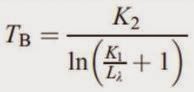
Step two converts the at-satellite radiance to blackbody temperature allowing kinetic temperature to be calculated in step three if land cover/use and emissivity data is available. Radiant (blackbody) temperature is calculated through the equation,

where:
TB = Radiant (blackbody) temperature
K1 and K2  = pre-launch calibration constants, found in various online sources for TM and ETM+ (found in metadata for Landsat 8)
L(lambda) = at-satellite radiance, calculated in step one


Screenshot of the model and equation used to convert the at-satellite image to a radiant temperature image. The Data Type was changed to Float Single for the output raster.


Screenshot of the radiant (blackbody) temperature image. Temperature information in this image is presented in degrees Kelvin. This image was opened in ArcMap and symbolized. Using the identify tool, an estimate of temperature was made for different land surface features. Lake Wissota was estimated at about 61 degrees Fahrenheit and a Chippewa Valley Regional Airport runway was estimated at about 101 degrees Fahrenheit.


Next, a Landsat TM image taken in the year 2011 of the same area was converted into a radiant (blackbody) temperature image through the same process as above. The two models were combined into one for efficiency.


Screenshot of the two models combined into one. The middle at-satellite radiance raster was designated Temporary Raster Only, as the specific image is not needed other than to produce the radiance (blackbody) temperature image.


The output image was opened in ArcMap and symbolized in the same fashion. An estimate of surface temperature for Lake Wissota was taken and compared to the value collected from the year 2000 ETM+ imagery. In 2000, Lake Wissota measured about 61 degrees Fahrenheit. In 2011, Lake Wissota measured about 74 degrees Fahrenheit. This 13 degree difference could be attributed to difference in season, water level, or differences in organic/pollution levels.

Finally, band 10 of a Landsat 8 TIRS image of Eau Claire and Chippewa Valley counties was converted into a radiant (blackbody) temperature image using the methods described above, opened in ArcMap, and made into a map of surface temperature in degrees Kelvin.


- Results -


Map of radiant temperature of western Wisconsin and southeastern Minnesota from Landsat ETM+ imagery taken in 2000.


Map of radiant temperature of western Wisconsin and southeastern Minnesota from Landsat TM imagery taken in 2011.


Map of radiant temperature of Eau Claire and Chippewa Valley counties from Landsat 8 TIRS imagery taken in 2014.


- Conclusion -

Thermal imagery from Landsat TM, ETM+, and TIRS was converted into radiant (blackbody) temperature images through a two step process using model maker in ERDAS. Another step would be needed to find actual kinetic temperatures for land surface features, however, this step fell outside the scope of this lab. By using the output images from this lab, surface temperature could be estimated and compared over time. This lab introduced key concepts and methodologies for extracting land surface temperatures from remotely sensed data.


- Sources -

Earth Resource Observation and Science Center, United States Geological Survey. (2000). Landsat ETM+

ESRI counties vector features. AOI file


Friday, September 12, 2014

Image Quality Assessment and Statistical Analysis


-Introduction-

Satellite imagery will often contain data redundancy which needs to be identified and removed before accurate analysis can be preformed. This image preprocessing can be accomplished through use of univariate statistics, multivariate statistics, and feature space plots. In this lab, feature space plots and correlation matrixes will be created to analyze bands in Landsat ETM+ and Quickbird satellite images to learn more about the practical uses of statistical analysis.


            • Screenshot of Landsat ETM+ imagery of Eau Claire, WI and the surrounding area


            • Screenshot of the Quickbird Imagery of the Florida Keys


            • Screenshot of the Quickbird Imagery of parts of Bangladesh


-Methods-

Programs: ERDAS IMAGINE 2013

Creation of Feature Space Plots

Navigate to Raster > Supervised > Feature Space Image. The "Create Feature Space Images" window will appear.


Image 1: Six bands will be analyzed in this Landsat ETM+ image. Fifteen feature space plots will be created through the unique pairing of bands 1, 2, 3, 4, 5, and 7. This image displays these band combinations. With " Output To Viewer" checked, the feature space plots were then displayed on the screen and shown in the Discussion section below.
 
 
Creation of Correlation Matrixes
To create a correlation matrix, the Model Maker tool was utilized. To open model maker navigate to Toolbox > Model Maker. A "New_Model" window will appear as well as a tool palette.

 
Image 2: Here is the first model created using the same Landsat ETM+ imagery as above. The model is rather simple with a raster connected to a function which in turn is connected to a matrix. Each of the three models followed this design. 
 
The matrixes created from the models needed to be opened in notepad, copied, and pasted (using the "Use Text Import Wizard" and checking the "Delimited" option) into excel for proper formatting. Further information on the statistical analysis is detailed in the Discussion section below.


-Discussion-

In determining data redundancy, visual interpretation through use of feature space plots and statistical analysis through use of correlation matrixes were utilized.

A feature space plot graphically illustrations the degree of correlation between two bands in satellite imagery by extracting the brightness values of each pixel and plotting their frequency. The brighter and "wider" a feature space plot, the higher the frequency of differing values, indicating low correlation. The darker and "narrower" a feature space plot, the lower the frequency of differing values, indicating high correlation.


Image 3: The fifteen feature space plots created from the Landsat ETM+ imagery. The yellow numbers were added with Photoshop for easy identification of band combinations.


Image 4: Narrow Feature Space Plot

From the feature space plots created, band combination 2 - 3, seen to the left, is an example of a narrow feature space plot. By visually examination, it can be determined that one of these bands could be eliminated from further analysis because they exhibit data redundancy. Data redundancy is another way of saying the bands portray similar information which could cause over- or underestimation of values in later analysis. Therefore, narrow feature space plots are undesirable.


Image 5: Wide Feature Space Plot


Band combination 4 - 5, seen to the right, is an example of a wide feature space plot. The amount of bright color in this plot indicates that the brightness values in the two bands have little correlation. This tells us there is little data redundancy and analyzing these bands together will give unique information. Wide feature space plots allow for accurate information to be gathered in later analysis and are therefore desirable.


After examining feature space plots, the analysis was taken a step further with the creation of correlation matrixes. The correlation of two bands is calculated by taking the covariance between the bands divided by the product of the bands standard deviation and will result in a coefficient varying between -1 and 1, with values close to 1 indicating data redundancy. If two bands are highly correlated their correlation coefficient must by equal to or greater than 0.95. When this occurs, one of the bands should be excluded to reduce error and computation costs of further analysis. In contrast, a low correlation coefficient indicates low correlation and unique information.

Three correlation matrixes were created in this lab. The first using Landsat ETM+ imagery and the others using Quickbird Imagery.


Table 1: Correlation Matrix of Landsat ETM+ Imagery
of Eau Claire, WI
In Table 1, it can be seen that band 2 has high correlation with band 1, with a coefficient near 0.926, and band 3, with a coefficient near 0.943. Nether of these coefficients exceed the threshold of 0.95 however, so a judgment call or preferably further analysis will be needed to determine if excluding Band 2 will be significant in reducing data redundancy.


Table 2: Correlation Matrix of Quickbird Imagery
of the Florida Keys
In Table 2, it can be seen that band 1 and band 2 have very high correlation, exceeding the threshold of 0.95 with a coefficient near 0.987. This indicates that one of these bands needs to be excluded to reduce data redundancy.


Table 3: Correlation Matrix of Quickbird Imagery
 of Bangladesh
In Table 3, it can be seen that, similarly to the last Quickbird image, bands 1 and 2 have high correlation exceeding the 0.95 threshold with a coefficient near 0.963. Again, one of these bands should be excluded from further analysis.


In determining which bands to use and which to exclude, it can be helpful to examine the rest of the matrix and determine if one of the bands in question has high correlation with another band. However, generally the type of analysis being preformed will determine which bands stay and which bands go when it comes to correlation. For example, if Landsat ETM+ imagery is used and bands 5 (NIR) and 1 (Visible Blue) show high correlation, it makes little sense to exclude band 5 if the goal of the analysis is vegetation identification (due to fundamental properties of plants). Using the same example, if the goal of the analysis is focused on water, it would make little sense to exclude band 1 (due to the high absorption of NIR radiation in water).


-Conclusion-

The visual results, in the form of feature space plots and correlation matrixes, can be seen in the Discussion section above. Creating, using and analyzing these graphical and statistical methods built on knowledge gained from the introductory from of this class to establish techniques for determining data redundancy in satellite imagery. Along with the removal of noise, the removal of data redundancy is an important part of preprocessing to insure the data collected will be accurate as possible.


-Sources-

Earth Resources Observation and Science Center, United States Geological Survey. (2011). Landsat ETM+

Global Land Cover Facility. (2012). Quickbird. www.landcover.org


Thursday, September 11, 2014

The Blog and the Blogger

This is an undergraduate student blog for Geography 438, Advanced Remote Sensing, taken at the University of Wisconsin Eau Claire. Posts will adhere to a technical report format detailing the goals, methods, and results of each lab exercise. Along with this information, general concepts will also be discussed as they pertain to each specific exercise.

My name is Lee Fox and I will be completing my bachelor's degree in geography this semester. I have made class blogs for Remote Sensing of the Environment (introductory), GIS I, and Geospatial Field Methods. Along with this blog, I will also be updating another blog this semester for GIS II. Over the last couple of years, I have learned to love geography for its simplicity and complexity. Each class has built on my ability to think spatially and through the medium of blogging, I hope to convey what I have learned and am currently learning.