Surface Temperature Extraction from Thermal Remote Sensing Data

-Introduction-

Thermal imagery records the emitted energy from land surface features and can be used to extract surface temperature information through a three step process.

1. Convert the thermal imagery to at-satellite spectral radiance
2. Convert the at-satellite spectral radiance to radiant (blackbody) temperature
3. Convert the radiant (blackbody) temperature to kinetic temperature

In this lab, the first two steps will be preformed to visually distinguish relative temperature differences and to estimate land surface temperature.

- Background -

Basics of thermal remote sensing:

• Thermal imagery represents emittance. This differs from the visible and IR bands which represent reflectance.
• The thermal band ranges from 3 to 14 micrometers. For reliable measurements, this range is reduced to 7 to 14 micrometers, due to atmospheric absorption of the emitted energy.
• Kinetic heat is the true temperature of a feature
• Radiant heat is the apparent heat (or what is physically felt) of a feature
• Thermal inertia is the ability of a feature to retain heat during the day and emit it during the night. Thermal inertia and temperature change have an inverse relationship.
• A blackbody is a hypothetical feature which absorbs all radiation and emits all radiation at the maximum amount for each wavelength for any temperature. This blackbody emittance is used in conjunction with emissivity to calculate kinetic heat.
• Stefan-Boltzman law: the amount of energy emitted by an object (blackbody) depends on the surface temperature of the object. (emittance will increase rapidly with increases in temperature)
• Wien's displacement law: the wavelength at which a blackbody reaches a maximum emission is inversely related to  its absolute temperature. (increases in blackbody temperature shifts wavelengths from long to short)
• Kirchoff's law: the ratio of emitted radiation to absorbed radiation flux is the same for all blackbodies at the same temperature. (land surface features will emit a certain proportion of energy emitted by a blackbody at the same temperature)
• Emissivity is the ratio between the actual emittance of a land surface feature and that of a blackbody at the same kinetic temperature. Values of emissivity range from 0 to 1. Land surface features with a high emissivity will radiate more energy.
• Path radiance is reflected and emitted radiation from non-target land surface features and the atmosphere. The values for this radiation need to be eliminated to collect accurate measurements.

- Methods -

ERDAS IMAGINE 2013 and ArcMap 10.2.2 was used to complete this lab.
Each model was created by navigating to Toolbox > Model Maker in ERDAS.


Step one removes atmospheric interference in the form of path radiance through the equation,

where:
L(lambda) = at-satellite radiance
DN = digital number = the thermal image
Grescale = Gain = (LMAX - LMIN)/(QCALMAX - QCALMIN), variables located in metadata
Brescale = Bias = LMIN

Screenshot of ETM+ imagery taken in the year 2000 of Western Wisconsin in band 62 (low gain). This image was used to visually identify land surface features of warmer and cooler temperature. Darker tones of gray represent cooler features and lighter tones of gray represent warmer features. The coolest features were rivers and lakes. The warmest features were urban and built up areas. Forested areas tended to fall in-between.

Screenshot of the model and equation used in step one to remove the atmospheric interference due to path radiance

Screenshot of the output at-satellite radiance image after the model was run.









Step two converts the at-satellite radiance to blackbody temperature allowing kinetic temperature to be calculated in step three if land cover/use and emissivity data is available. Radiant (blackbody) temperature is calculated through the equation,

where:
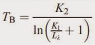
TB = Radiant (blackbody) temperature
K1 and K2  = pre-launch calibration constants, found in various online sources for TM and ETM+ (found in metadata for Landsat 8)
L(lambda) = at-satellite radiance, calculated in step one

Screenshot of the model and equation used to convert the at-satellite image to a radiant temperature image. The Data Type was changed to Float Single for the output raster.

Screenshot of the radiant (blackbody) temperature image. Temperature information in this image is presented in degrees Kelvin. This image was opened in ArcMap and symbolized. Using the identify tool, an estimate of temperature was made for different land surface features. Lake Wissota was estimated at about 61 degrees Fahrenheit and a Chippewa Valley Regional Airport runway was estimated at about 101 degrees Fahrenheit.







Next, a Landsat TM image taken in the year 2011 of the same area was converted into a radiant (blackbody) temperature image through the same process as above. The two models were combined into one for efficiency.

Screenshot of the two models combined into one. The middle at-satellite radiance raster was designated Temporary Raster Only, as the specific image is not needed other than to produce the radiance (blackbody) temperature image.










The output image was opened in ArcMap and symbolized in the same fashion. An estimate of surface temperature for Lake Wissota was taken and compared to the value collected from the year 2000 ETM+ imagery. In 2000, Lake Wissota measured about 61 degrees Fahrenheit. In 2011, Lake Wissota measured about 74 degrees Fahrenheit. This 13 degree difference could be attributed to difference in season, water level, or differences in organic/pollution levels.

Finally, band 10 of a Landsat 8 TIRS image of Eau Claire and Chippewa Valley counties was converted into a radiant (blackbody) temperature image using the methods described above, opened in ArcMap, and made into a map of surface temperature in degrees Kelvin.


- Results -

Map of radiant temperature of western Wisconsin and southeastern Minnesota from Landsat ETM+ imagery taken in 2000.

 

Map of radiant temperature of western Wisconsin and southeastern Minnesota from Landsat TM imagery taken in 2011.

Map of radiant temperature of Eau Claire and Chippewa Valley counties from Landsat 8 TIRS imagery taken in 2014.









- Conclusion -

Thermal imagery from Landsat TM, ETM+, and TIRS was converted into radiant (blackbody) temperature images through a two step process using model maker in ERDAS. Another step would be needed to find actual kinetic temperatures for land surface features, however, this step fell outside the scope of this lab. By using the output images from this lab, surface temperature could be estimated and compared over time. This lab introduced key concepts and methodologies for extracting land surface temperatures from remotely sensed data.


- Sources -

Earth Resource Observation and Science Center, United States Geological Survey. (2000). Landsat ETM+

ESRI counties vector features. AOI file

Image Quality Assessment and Statistical Analysis

-Introduction-

Satellite imagery will often contain data redundancy which needs to be identified and removed before accurate analysis can be preformed. This image preprocessing can be accomplished through use of univariate statistics, multivariate statistics, and feature space plots. In this lab, feature space plots and correlation matrixes will be created to analyze bands in Landsat ETM+ and Quickbird satellite images to learn more about the practical uses of statistical analysis.

• Screenshot of Landsat ETM+ imagery of Eau Claire, WI and the surrounding area

• Screenshot of the Quickbird Imagery of the Florida Keys

• Screenshot of the Quickbird Imagery of parts of Bangladesh

-Methods-

Programs: ERDAS IMAGINE 2013

Creation of Feature Space Plots

Navigate to Raster > Supervised > Feature Space Image. The "Create Feature Space Images" window will appear.

Image 1: Six bands will be analyzed in this Landsat ETM+ image. Fifteen feature space plots will be created through the unique pairing of bands 1, 2, 3, 4, 5, and 7. This image displays these band combinations. With " Output To Viewer" checked, the feature space plots were then displayed on the screen and shown in the Discussion section below.

 

 

Creation of Correlation Matrixes

To create a correlation matrix, the Model Maker tool was utilized. To open model maker navigate to Toolbox > Model Maker. A "New_Model" window will appear as well as a tool palette.

 

Image 2: Here is the first model created using the same Landsat ETM+ imagery as above. The model is rather simple with a raster connected to a function which in turn is connected to a matrix. Each of the three models followed this design. 

 

The matrixes created from the models needed to be opened in notepad, copied, and pasted (using the "Use Text Import Wizard" and checking the "Delimited" option) into excel for proper formatting. Further information on the statistical analysis is detailed in the Discussion section below.

-Discussion-

In determining data redundancy, visual interpretation through use of feature space plots and statistical analysis through use of correlation matrixes were utilized.

A feature space plot graphically illustrations the degree of correlation between two bands in satellite imagery by extracting the brightness values of each pixel and plotting their frequency. The brighter and "wider" a feature space plot, the higher the frequency of differing values, indicating low correlation. The darker and "narrower" a feature space plot, the lower the frequency of differing values, indicating high correlation.

Image 3: The fifteen feature space plots created from the Landsat ETM+ imagery. The yellow numbers were added with Photoshop for easy identification of band combinations.




Image 4: Narrow Feature Space Plot

From the feature space plots created, band combination 2 - 3, seen to the left, is an example of a narrow feature space plot. By visually examination, it can be determined that one of these bands could be eliminated from further analysis because they exhibit data redundancy. Data redundancy is another way of saying the bands portray similar information which could cause over- or underestimation of values in later analysis. Therefore, narrow feature space plots are undesirable.




Image 5: Wide Feature Space Plot

Band combination 4 - 5, seen to the right, is an example of a wide feature space plot. The amount of bright color in this plot indicates that the brightness values in the two bands have little correlation. This tells us there is little data redundancy and analyzing these bands together will give unique information. Wide feature space plots allow for accurate information to be gathered in later analysis and are therefore desirable.



After examining feature space plots, the analysis was taken a step further with the creation of correlation matrixes. The correlation of two bands is calculated by taking the covariance between the bands divided by the product of the bands standard deviation and will result in a coefficient varying between -1 and 1, with values close to 1 indicating data redundancy. If two bands are highly correlated their correlation coefficient must by equal to or greater than 0.95. When this occurs, one of the bands should be excluded to reduce error and computation costs of further analysis. In contrast, a low correlation coefficient indicates low correlation and unique information.

Three correlation matrixes were created in this lab. The first using Landsat ETM+ imagery and the others using Quickbird Imagery.





Table 1: Correlation Matrix of Landsat ETM+ Imagery
of Eau Claire, WI

In Table 1, it can be seen that band 2 has high correlation with band 1, with a coefficient near 0.926, and band 3, with a coefficient near 0.943. Nether of these coefficients exceed the threshold of 0.95 however, so a judgment call or preferably further analysis will be needed to determine if excluding Band 2 will be significant in reducing data redundancy.







Table 2: Correlation Matrix of Quickbird Imagery
of the Florida Keys

In Table 2, it can be seen that band 1 and band 2 have very high correlation, exceeding the threshold of 0.95 with a coefficient near 0.987. This indicates that one of these bands needs to be excluded to reduce data redundancy.






Table 3: Correlation Matrix of Quickbird Imagery
 of Bangladesh

In Table 3, it can be seen that, similarly to the last Quickbird image, bands 1 and 2 have high correlation exceeding the 0.95 threshold with a coefficient near 0.963. Again, one of these bands should be excluded from further analysis.



In determining which bands to use and which to exclude, it can be helpful to examine the rest of the matrix and determine if one of the bands in question has high correlation with another band. However, generally the type of analysis being preformed will determine which bands stay and which bands go when it comes to correlation. For example, if Landsat ETM+ imagery is used and bands 5 (NIR) and 1 (Visible Blue) show high correlation, it makes little sense to exclude band 5 if the goal of the analysis is vegetation identification (due to fundamental properties of plants). Using the same example, if the goal of the analysis is focused on water, it would make little sense to exclude band 1 (due to the high absorption of NIR radiation in water).


-Conclusion-

The visual results, in the form of feature space plots and correlation matrixes, can be seen in the Discussion section above. Creating, using and analyzing these graphical and statistical methods built on knowledge gained from the introductory from of this class to establish techniques for determining data redundancy in satellite imagery. Along with the removal of noise, the removal of data redundancy is an important part of preprocessing to insure the data collected will be accurate as possible.


-Sources-

Earth Resources Observation and Science Center, United States Geological Survey. (2011). Landsat ETM+

Global Land Cover Facility. (2012). Quickbird. www.landcover.org

The Blog and the Blogger

This is an undergraduate student blog for Geography 438, Advanced Remote Sensing, taken at the University of Wisconsin Eau Claire. Posts will adhere to a technical report format detailing the goals, methods, and results of each lab exercise. Along with this information, general concepts will also be discussed as they pertain to each specific exercise.

My name is Lee Fox and I will be completing my bachelor's degree in geography this semester. I have made class blogs for Remote Sensing of the Environment (introductory), GIS I, and Geospatial Field Methods. Along with this blog, I will also be updating another blog this semester for GIS II. Over the last couple of years, I have learned to love geography for its simplicity and complexity. Each class has built on my ability to think spatially and through the medium of blogging, I hope to convey what I have learned and am currently learning.