Advanced Classifiers

- Introduction -

Multiple classification methods have been used throughout the semester including supervised, unsupervised, and fuzzy logic, each having its advantages and disadvantages. However, none of these methods has created a classification with suitable accuracy for use in further analysis. Two advanced classifiers, expert tree and neural network, have the potential to reach a level that exceeds the minimum accepted overall accuracy for classified images (85%). Both of these classifiers are used and discussed in this lab exercise.

- Background -

Expert tree, or expert system, classification employs ancillary data to improve on an already classified image. An expert system is comprised of three parts: hypotheses, rules, and conditions. A hypothesis is a terminal (or intermediate) informational class (such as water or forest) and is connected to a rule. Rules are written by the analyst to allow specific communication between the hypotheses and the previously classified image and ancillary data. These rules can be implicit, explicit, conditional or Boolean. Conditions are statements that define a new classification based on its connected rule(s) and hypothesis. The types of ancillary data that can be used are numerous and include zoning, elevation, vegetation, temperature, and soil data. Extensive knowledge of the study area is recommended.

Neural Networks attempt to simulate the human brain when classifying an image. Through back-propagation, a number of iterations pass back and forth from input layers to a result until a user defined error threshold is reached. The connections between the input layers and the result are called hidden layers. As iterations pass through the hidden layers, weights are developed and modified in response to the error present in the currently generated result. Reflective remote sensing data and ancillary data are used as inputs for neural networks and the result can be modified by changing the parameters of then neural network like training rate and training momentum.

- Methods -



Image 1: The finished classification tree. Hypotheses > Rules > Conditions

 


A previously classified image of Eau Claire, Chippewa Falls, and the City of Altoona, WI was enhanced through use of census and elevation data in an expert system classification with  ERDAS IMAGINE 2010. The classification tree was created by navigating to Raster > Knowledge Engineer. In the knowledge engineer, the hypotheses, rules, and conditions (variables) were added. First, arguments were created to relate five desired terminal classes to the classified image. Then ancillary data was incorporated by creating 3 arguments and counter arguments to reclassify certain erroneously classified land cover. Counter arguments were then added for the terminal classes effected by the 3 arguments created through the ancillary data (residential, green vegetation, and agriculture). The finished classifier (Image 1) was then used to performed expert system classification be selecting 'Knowledge Classifier' in the Knowledge Engineer window. The classifier created 8 classes based on the 8 arguments in the classification tree. The 8 classes were then appropriately merged into the desired 6 terminal classes and made into a map (Map 1).

Image 2: Graph of the RMSE error
for each iteration of the neural
network classifier

A simple classification for a Landsat TM image of the University of Northern Iowa was created through a neural network using ENVI software. Three homogenous regions of interest (ROIs) were created for bare soil, green vegetation, and snow. These ROIs were used to classify the image and the number of iterations was increased to ensure the neural network would reach the error threshold and finish (Image 2).






- Results -

 

Map 1: Result of the expert system classification

 

Image 3: Result of the neural network classification. Blue is bare soil,
green is green vegetation, and red is snow.

 

- Discussion -

The expert system classification was able to increase the accuracy of the classification as well as the number of informational classes. The accuracy increase is seen in green vegetation, agriculture, and urban areas as those were the classes effected by the introduction of ancillary data. Small areas of urban classification are often seen in forested areas, known as the 'salt and pepper effect', and more ancillary data would need to be included to increase the accuracy of the forest classification. The urban classification was enhanced by creating a new class, other urban, through population density data. The distinction between urban and other urban attempts to separate residential areas and other urban features (airport, shopping mall, etc).

The concept of the neural network is intriguing but its use can be limited due to the desired level of complexity and size of the study area in relation to computer resources. The classification developed through the neural network method was simple but seemed to be effective. Just like with other classified images, a neural network classification could be used as input in an expert system to further its accuracy.

- Conclusion -

Two advanced classifiers were used in this lab exercise which produced better classifications (through visual analysis) than the standard classifiers used earlier in the semester. Neural networks attempt to simulate the human brain by relating and processing data many times. An expert system classifier can increase the accuracy of a previously classified image by removing erroneous classifications and creating new sub-classes.

- Sources -

Department of Geography, University of Northern Iowa. Quickbird imagery.

Earth Resources Observation and Science Center, USGS. Landsat imagery.

United States Census Bureau. Census population density data.

Spectral Mixture Analysis and Fuzzy Classification

- Introduction -

Advanced classifiers were developed to increase the accuracy of image classification. A type of advanced classifier, sub-pixel, can be used to solve the mixed pixel problem that occurs in remotely sensed imagery when surface features are smaller that the sensor's instantaneous field of view (IFOV). The mixed pixel problem results in a composite signature (multiple land covers) for one pixel making hard classification difficult and introducing error into the classified image. Qualitative assessments of fractional images produced through spectral mixture analysis (SMA) (otherwise known as linear spectral unmixing) and a hardened fuzzy classification of the same Landsat ETM+ image of Eau Claire and Chippewa Counties, WI will be discussed in this post.

- Background -

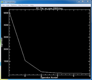
To perform SMA, endmemebers (specific land covers) are collected from the vertices of transformed image feature space of a principle component (PC) or minimum noise fraction (MNF) image of the study area. A PC image will have multiple bands that contain decreasing amounts of unique information which can be interpreted through use of Eigen values (Figure 1). The endmembers are then applied through a constrained least-squares regression to produce fractional images. The factional images display pure areas of a specific land cover in white, areas with none of the specific land cover in black, and a range of gray tones for areas with a mix of the specific land cover and others. An RMS image is also created which displays areas of higher error in white and lower error in black, with gray tones in-between. Once the RMS error is acceptable the factional images can be combined and used in a classifier to create a classified image.

Fuzzy classification is performed in a similar fashion to supervised classification in that training samples must be collected from the image. However, the requirements for training samples for fuzzy classification differ greatly from that of supervised. For fuzzy classification, training samples should contain both homogenous and heterogeneous signatures and contain between 150-300 pixels. The output of fuzzy classification will produce multiple classified images. The first image will show the most probably classification for each pixel. The second image will show the second most probable classification for each pixel and the trend continues for the rest of the images. Each pixel will have associated membership grades for each class which range in value from 0 to 1. The soft classification produced through fuzzy classification can be hardened into a single hard classified image by setting the highest membership grade of a pixel to 1 or through use of fuzzy convolution.

- Methods -

Figure 1: Eigen values for each band (Eigenvalue number) of
the PC image. Higher Eigen values indicate
 more unique information.

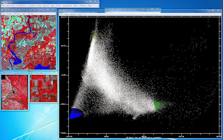
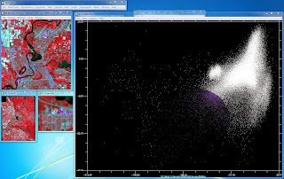
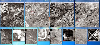
ENVI software was used to perform SMA on imagery of Eau Claire and Chippewa Counties, WI. The image was converted into a PC image with 6 bands. Three endmembers, water, agriculture, and forest, were collected from the transformed image feature space plot of bands 1 and 2 of the PC image and one endmember, urban, was collected from bands 3 and 4. These endmembers were then saved as a ROI file and used to create four fractional images through SMA corresponding to each endmember. A classified image was not created with this method but the fractional images and RMS error image were qualitatively analyzed.

 

Figure 2: Endmember collection from the transformed image feature space
plot of bands 1 and 2 of the PC image.

 

 

Figure 3: Endmember collection from the transformed image feature space
plot of bands 3 and 4 of the PC image.

 

Figure 4: The fractional images for each of the endmembers

 

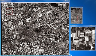
Figure 5: RMS error image

Fuzzy classification was performed with ERDAS IMAGINE software. Appropriate training samples for water, urban, agriculture, bare soil, and forest were collected, merged, and saved. These resulting 5 training samples were then used in a fuzzy classification of the same image of Eau Claire and Chippewa Counties, WI used earlier. The five fuzzy classified images were then hardened using a fuzzy convolution window.

- Results -

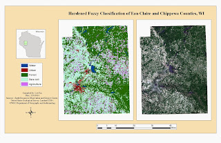
Map 1: The hardened fuzzy classification

- Discussion -

Four fractional images for water, agriculture, bare soil, and urban features were generated through SMA. Each fractional image, aside from urban, makes sense when visually examining the fractional images against a color composite image and Google Earth historical imagery. The fractional image for water highlights water features and areas of higher moisture, like riparian vegetation, and displays urban areas in black or dark tones of gray. Areas of bare soil display a wide range of values from bright white to dark gray. The fractional images for agriculture and bare soil are interesting to compare. Both de-emphasis water and urban features and seem to be opposites of each other in regards to highlighting vegetated and non vegetated land cover. Plots of land that are highlighted in the agriculture fractional image are not in the bare soil fractional image and vice versa. Forested area is highlighted in the agriculture fractional image more so than the other three. For the urban fractional image, all land covers, except for bare soil, are highlighted in white or light tones of gray. Urban features are mostly white which is desirable but too much agriculture, forest, and water are highlighted as well. This could be due to a lower quality endmember taken for urban features when compared to the other endmembers, which can be seen in Figures 2 and 3.

 The RMS error image indicates less error for water and urban features, more error for agriculture and forested areas, and the most error for bare soil. This demonstrates that just because a fractional image for a land cover makes sense in comparison to that specific land cover, this does not mean that there is no error associated with that land cover in comparison to other land covers. In the water fractional image, areas of bare soil are commonly highlighted. This error plus the small amounts of error (dark tones of gray) for bare soil in the fractional images for urban and agriculture can add up. The small amount of error associated with urban features makes sense because in every fractional image, aside from the one for urban, urban features are shown in black or dark tones of gray. The same can be said for water, even though water features are highlighted in the urban fractional image as well as the water fractional image.

Qualitative confidence building was performed on the classified image produced through the fuzzy classification method. Compared to the qualitative assessments of the images produced through unsupervised and supervised classification of the same area, the fuzzy classification method did a much better job at representing actual land use/land cover (LULC) (Map 1). The distribution of urban areas are far more appropriate and the mix-up between what constitutes bare soil was re-worked. For this classification, fallow agriculture, bare soil, and areas of sparse vegetation (e.g. grass fields, scrublands) were all lumped together into the bare soil class. This helped me find appropriate training samples to accurately model the different LULC types. However, this also means that bare soil is overestimated, but this is an inevitable fact given the requirement of five LULC classes. The training samples were modified three times before generating the final image. Modifying the training samples further could no doubt have improved on the accuracy of the fuzzy classification further.

- Conclusion -

Using SMA provides an opportunity to visualize specific land covers as pure and mixed areas, as well as provides an error assessment. The information gained by selecting quality endmembers can be used to classify an image or enhance a classification. The qualitative confidence given to the classified image produced through fuzzy classification is far greater than that of the classified images produced through unsupervised and supervised methods. The ability of fuzzy classification to determine membership grades for LULC classes per pixel allows for the classified image to more accurately represent the landscape by combating the mixed pixel problem.

- Sources -

Earth Resources Observation and Science Center, United States Geological Survey (USGS). Landsat 7 (ETM+) imagery.

Environmental Systems Research Institute (ESRI). Geodatabase (2013) US Census Data. Accessed through UWEC Department of Geography and Anthropology.